Excel Practice 1

Since Microsoft Excel is widely used in industry, and we are using Microsoft Windows, we will focus on Excel going forward. There are many similarities across spreadsheet software, so the skills we are learning can be translated to other software and apps. The following ‘Practice It’ assignments are designed to be completed using Microsoft Excel in Office 365 on a PC with Windows 10 or higher.

We will use Excel to perform complex calculations, analyze data so that we can make intelligent decisions, and create visually interesting charts and graphs that help us understand the data. Since Excel is used for Data Analysis, it is best to use a keyboard and mouse or touchpad rather than the touchscreen.

In Excel, data is stored in a cell. Cell content is anything that is stored in the cell and can be either a constant value or a formula. The most commonly used values are text values and number values. Values can also be a date or time. A text value is also referred to as a label.

Prefer to watch and learn? Check out this video tutorial:

Complete the following Practice Activity and submit your completed project.

For our first assignment in Excel, we will create a spreadsheet with monthly expenses. This spreadsheet will provide us with an overall picture of our financial health by helping us understand where we are spending our hard-earned money. We will start with a new blank Excel Spreadsheet.

1. Start Excel. Click Blank Workbook.
2. Select File, Save As, Browse, and then navigate to your Excel folder on your NSCC OneDrive or other location where you save your files. Name the workbook as Yourlastname_Yourfirstname_Excel_Practice_1.
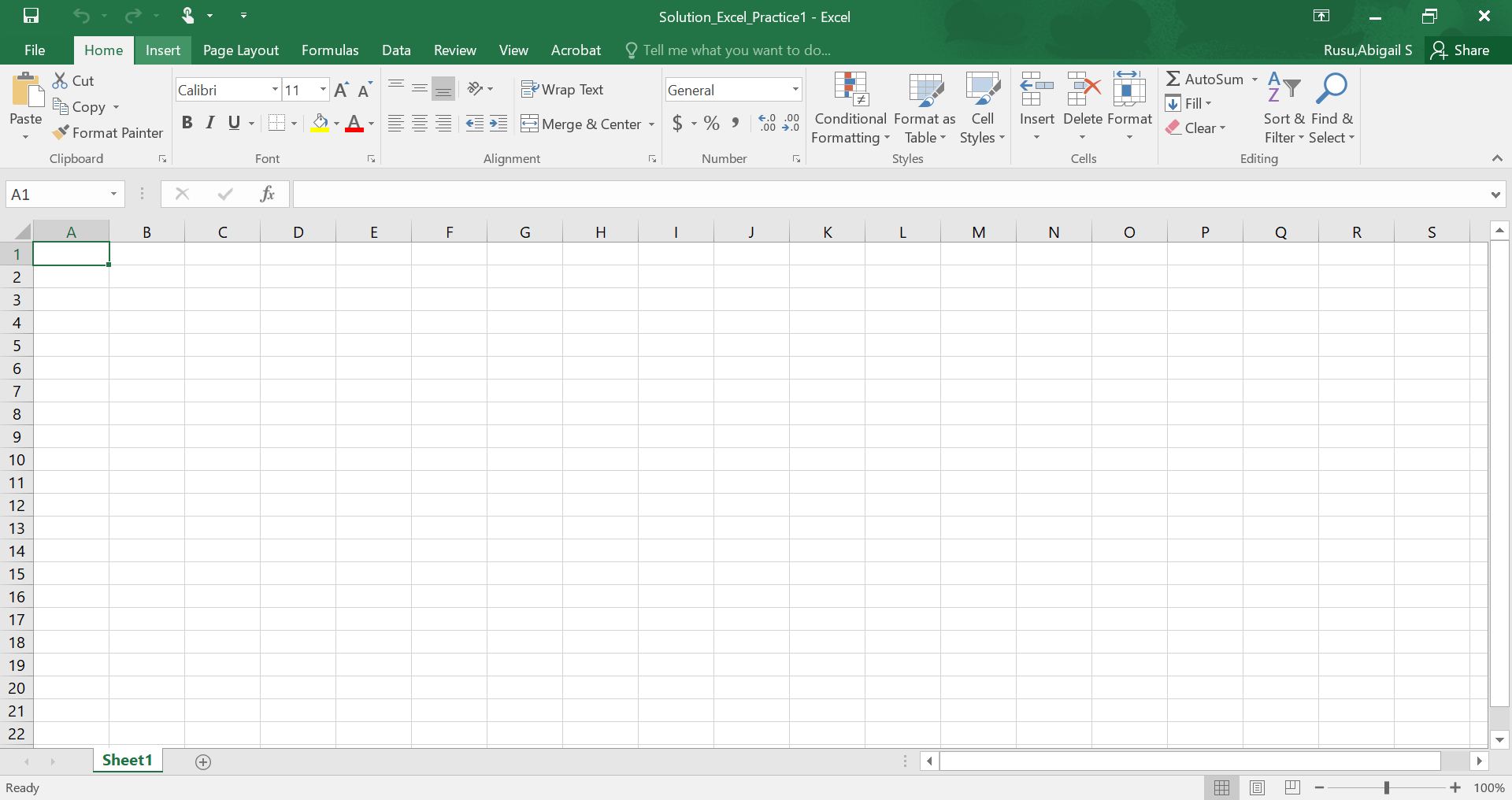
3. Take a moment to locate the following components of the Excel workbook window. Notice how Columns are lettered and Rows are numbered. The intersection of a row and column is a cell. The active cell in the image is A1.
4. Notice the vertical and horizontal scroll bars. Use the arrows to practice scrolling on the page.
5. In cell A1, type “My Budget By Month” and press Enter.
6. In cell A2 Type “For the First Quarter” and press Enter.
7. In the Name Box, change A3 to A4 and then press Enter. Notice how the active cell changed to A4.
8. Starting in cell A4, Type each of the following (excluding the circle bullets), pressing Enter after each:
   • Housing
   • Groceries
   • Utilities
   • Misc Expenses
   • Monthly Total
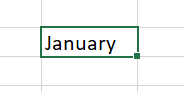
9. In cell B3, type January and press Enter.
10. Select cell B3 and use the fill handle to drag to cell D3. Notice how the names of the months automatically generate. The fill handle enables auto fill, which generates and extends a series of values into adjacent cells based on the value of other cells.

1. Adjust the column width for column A to Width 18.71 (136 pixels) by dragging the right boundary (between columns A and B) to the right.
2. Select the range B3:D3 and center the text.

Note: A range in Excel is two or more cells on a worksheet that are adjacent (next to each other) or nonadjacent (not next to each other). To select nonadjacent ranges, use the CTRL key on your keyboard.

1. In cell B4, type 1200 and enter the remaining numbers as shown: